はじめに

tidymodelsに属するparsnipパッケージを用いて機械学習を行った場合、大本のパッケージで学習した場合と異なる構造のオブジェクトが返ります。例えばxgboost::xgboost関数で学習した結果はxgb.Boosterクラスを持つオブジェクトです。一方でparsnip::fit関数を用いてXGBoostの学習を行った結果は、_xgb.Boosterクラスとmodel_fitクラスを持つオブジェクトです。

このため、後者はxgb.Boosterクラス用に用意された様々な関数を適用することができません。利用できない関数には、変数重要度を計算するxgboost::xgb.importance関数や、Partial Dependence Plotを行うpdp::partialなどがあります。これらはブラックボックスモデルなXGBoostの結果を解釈する上で非常に重要な関数です。簡単に使える方法を探ることにしました¹。

結論としては学習結果の"fit"要素が、xgboost本来の学習結果ですので、これを取り出せば様々な関数を利用できます。というわけで試してみましょう。

pacman::p_load(tidymodels, xgboost, pdp, dplyr)

XGBoostによる学習

ggplot2::diamondsデータセットについて、価格を予想するモデルを構築します。

# 1割をテストデータにする
set.seed(71)
i <- rsample::initial_split(ggplot2::diamonds, p = .9)

# 前処理方法を定義
rec <- training(i) %>%
  recipes::recipe(price ~ .) %>%
  recipes::step_ordinalscore(recipes::all_nominal()) %>%
  recipes::step_log(price)

prep <- recipes::prep(rec)

# 前処理方法を元に訓練データとテストデータを作成
tr <- juice(prep)
te <- bake(prep, testing(i))

# 学習
set.seed(71)
fit_xgb <- boost_tree("regression") %>%
  set_engine("xgboost") %>%
  fit(price ~ ., data = tr)

ここで、dplyr::glimpse(fit_xgb)すると、学習結果の構造を見ることができます。

xgboostパッケージ本来の出力結果と比較したい場合には、parsnip::xgb_train(x = tr %>% select(-Price), y = tr$Price)と比較してみて下さい。 fit_xgb$fitと同じ構造をしていることが分かります。

Variable Importance Plot (VIP)

学習結果を元に、変数重要度 (variable importance; VI) を計算してみましょう。これにはxgboost::xgb.importance関数を用います。 xgboost::xgb.importance関数はxgb.Boosterクラスオブジェクトを受けとるように設計されているので、fit_xgbそのものではなく、fit_xgb$fitを食わせてやりましょう。

すると、幅 (y) と、次いでカラット (carat) が価格に大きく影響することが分かります。

vi <- fit_xgb$fit %>%
  xgboost::xgb.importance(model = .) %>%
  print
#>    Feature         Gain      Cover  Frequency
#> 1:       y 5.411260e-01 0.13881580 0.11320755
#> 2:   carat 3.959879e-01 0.23607853 0.11725067
#> 3: clarity 2.185543e-02 0.20602836 0.27088949
#> 4:       x 1.798093e-02 0.10747288 0.09029650
#> 5:       z 1.301997e-02 0.04969059 0.04986523
#> 6:   color 8.731771e-03 0.16406459 0.21698113
#> 7:     cut 9.375364e-04 0.05300730 0.04312668
#> 8:   depth 3.103671e-04 0.03613783 0.07412399
#> 9:   table 5.006207e-05 0.00870413 0.02425876
xgboost::xgb.ggplot.importance(vi)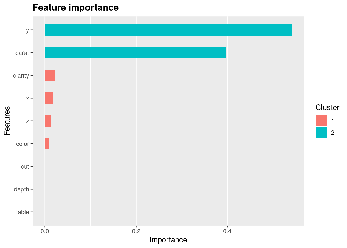

Partial Dependence Plot (PDP)

変数重要度が最も高いのは幅 (y) ですが、なんとなくカラット (carat) の方がイメージしやすいので、カラット (carat) についてPDPを可視化してみます。

pdp::partial関数もparsnip::fit関数の結果を受け取れないので、fit_xgb$fitを食わせます。計算時間を節約するため、train引数には訓練データの2割を与えることにしました。 pred.varには注目したい変数であるcaratを指定します。

set.seed(71)
tr_mini <- tr %>%
  select(-price) %>%
  initial_split(.2) %>%
  training()
pdp::partial(
  fit_xgb$fit, train = te %>% select(-price),
  pred.var = "carat",
  ice = TRUE, # 下図黒線としてIndividual Conditional Expectationを表示するか。
  plot = TRUE,
  plot.engine = "ggplot"
)

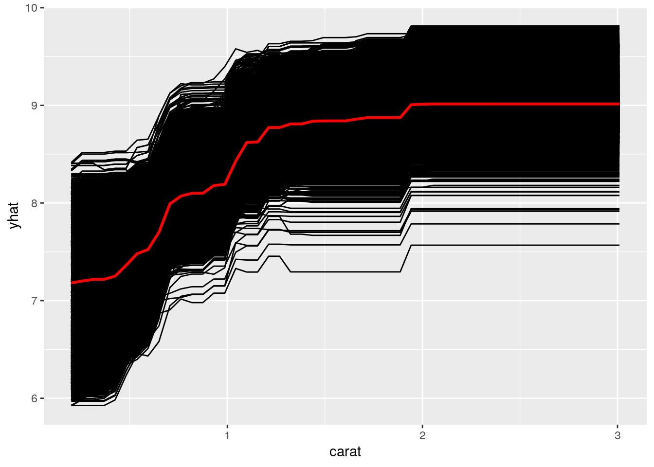
どうやら、2カラット以上では、大きさだけで価格が決まらなくなるようです。

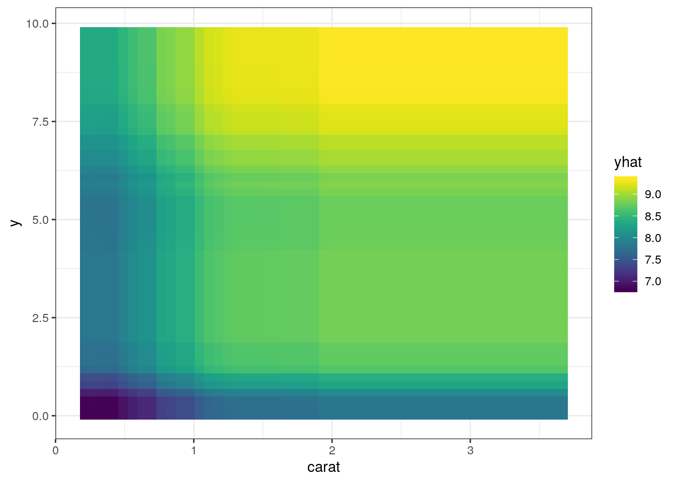
yにも注目して2変量を用いたPDPを作成してみましょう。すると、同じ大きさでも幅広なダイヤモンドの方が高値になる傾向が伺えます。大きなダイヤモンドは指輪にする時に、楕円状のテーブルを持っていた方が良いのかも知れません。

pdp::partial(
  fit_xgb$fit, train = tr_mini,
  pred.var = c("carat", "y"),
  ice = FALSE,
  plot = TRUE,
  plot.engine = "ggplot"
)

可視化で得られた考察を反映する

大きなダイヤモンドは指輪にする時に、楕円状のテーブルを持っていた方が良いのかも知れません。

と考えたので、縦横比を特徴量として追加してみましょう。

prep2 <- rec %>%
  recipes::step_mutate(y_per_x = y / x) %>%
  recipes::prep(train = rsample::training(i))
tr2 <- recipes::juice(prep2)
te2 <- recipes::bake(prep2, rsample::testing(i))
fit_xgb2 <- boost_tree("regression") %>%
  set_engine("xgboost") %>%
  fit(price ~ ., data = tr2)

そしてmetricsを計算し、前回の学習結果と比較してみます。

# 今回の学習結果のmetrics
predict(fit_xgb2, te2) %>%
  mutate(truth = te2$price) %>%
  metrics(.pred, truth)
#> # A tibble: 3 x 3
#>   .metric .estimator .estimate
#>   <chr>   <chr>          <dbl>
#> 1 rmse    standard      0.103 
#> 2 rsq     standard      0.991 
#> 3 mae     standard      0.0759

# 前回の学習結果のmetrics
predict(fit_xgb, te) %>%
  mutate(truth = te$price) %>%
  metrics(.pred, truth)
#> [00:58:56] WARNING: amalgamation/../src/objective/regression_obj.cu:152: reg:linear is now deprecated in favor of reg:squarederror.
#> # A tibble: 3 x 3
#>   .metric .estimator .estimate
#>   <chr>   <chr>          <dbl>
#> 1 rmse    standard      0.108 
#> 2 rsq     standard      0.990 
#> 3 mae     standard      0.0835

僅かながら、rmseとmaeは減少し、rsqは上昇しました。読みがあたりましたね！